imorbel

Orbital constraints for linear motion of directly imaged planets, enter values below, submit, and wait (briefly) for the results.

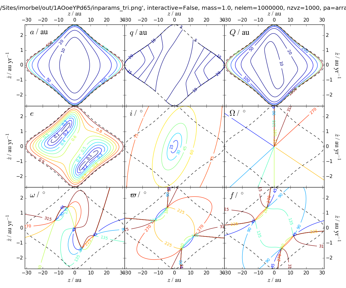
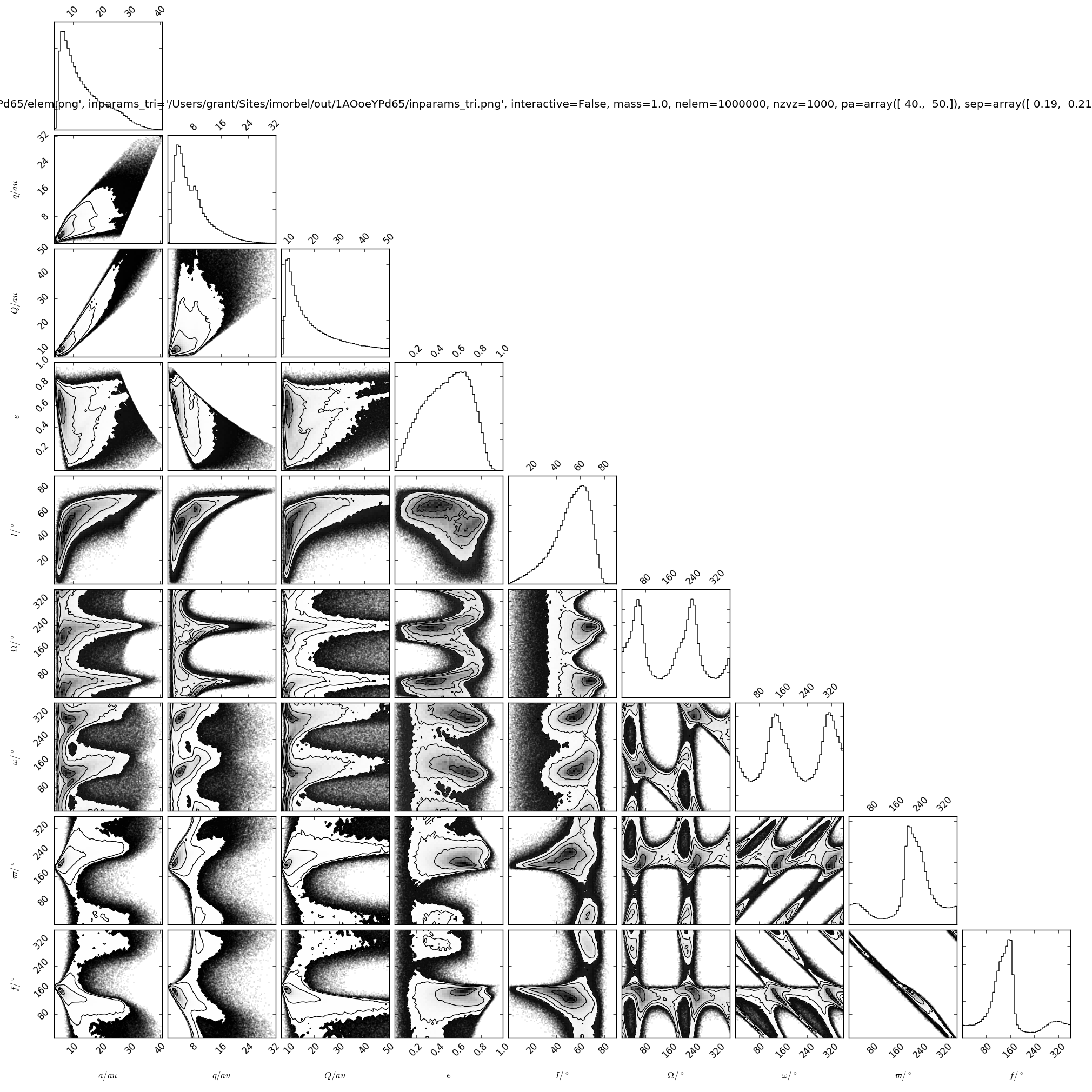
The plots displayed below show:

• The allowed ranges of the two unconstrained parameters of the companion (z and vz), and the orbital elements that result at each point in this 2d parameter space. Bound orbits lie inside the dashed lines. The "x" direction, where the ascending node is measured from, is with respect to the vector pointing to the companion from the star. Because the angle phi is restricted to 0-180deg, any object moving clockwise on the sky has it's z axis reversed, so the angles need to be converted as 360deg - angle.
• Samples from this parameter space, presented as a series of 2d plots of orbital elements (including the pericenter and apocenter distances q and Q, and longitude of periastron curlypi). The samples are restricted to bound orbits (e<1) and can be further restricted by setting the maximum apocenter distance (Q). In the parlance of other models that derive orbital constraints by MCMC, the resulting distributions are what would result from uniform priors in z and vz. The priors used are arbitrary, so the posterior distributions should not be taken as an indication of likely orbits.
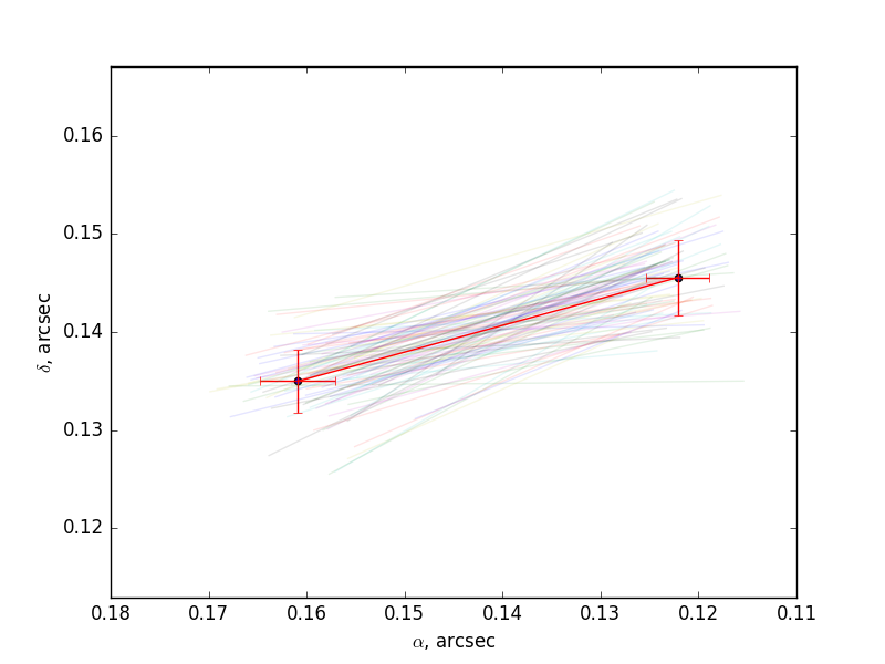
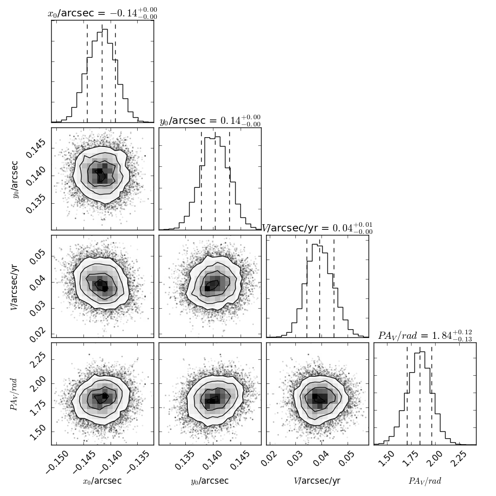
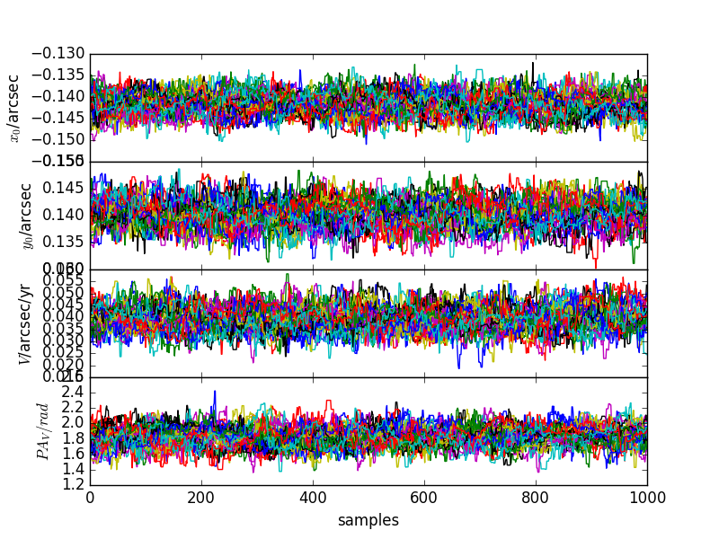
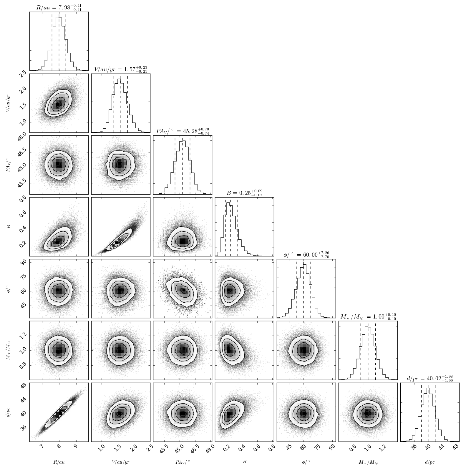
• When uncertainties are included, plots showing 1) the input astrometry and samples from the MCMC chains fitting them, 2) these samples in a corner plot, 3) the chains themselves, and 4) these samples converted into the quantities used as input for the best fit shown in the z/vz plot, and the samples used for the element plot.

For further details on the method see Pearce, Wyatt, & Kennedy (2015).

Uncertainties | No uncertainties

Additional plots are shown below that show how the astrometry is converted into input samples for deriving the elements.

Enter parameters here and click submit. Increasing N z/vz and N elem gives a smoother sampling in the element plot.